DataScience310

For this project, I choose the country of Slovakia for the sake of research. I originally had gone with the country of Nepal like in the last project however due to the large area I was unable to complete the models. I continued to get errors due to the raster sizes, however switching the countries solved this problem. Slovakia is a central European nation which borders Austria and the Czech Republic in the west, Poland to the north, Hungary to the south and Ukraine to the east. Much of the country is mountainous with the Tatras and the Fatra, and the Danube river forms a natural border between Slovakia and Hungary. These are important variations which likely account for differences in the data. In the middle of the country there are many mountains which contribute to the sparse population in the area. Further, the Danube River and the capital of Bratislavia in the west account for a large population in the maps. Further the city of Košice in the southwest is a major population center. To examine this country two machine learning methods were used, linear regression and random forest. Before examining the models, one must examine the data collected.

In the project, the data collected came from a few sources, GADM ADMs and Worldpop. From this data, the gadm36_SVK_0.shp and gadm36_SVK_2.shp files were used along with the esaccilc dst 011, 040, 130, 140, 150, 160, 190, 200, water, slope, topo, night time light(ntl), and population data to create a list. The sums of these rows was then used for the data used in the model. The data is the same across the two models. With an understanding of the data preprocessing, it is time to discuss the individual models and compare them.

The first model to be examined is the linear regression. Below are some graphics taken from the model.

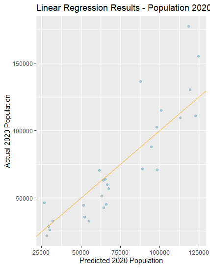
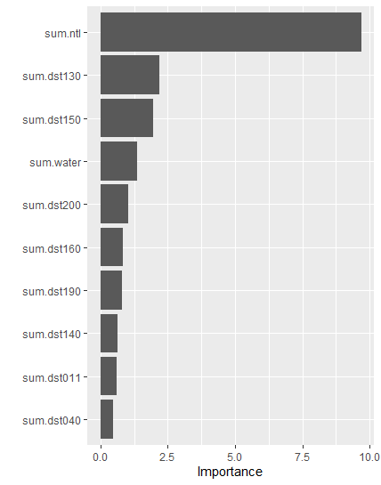
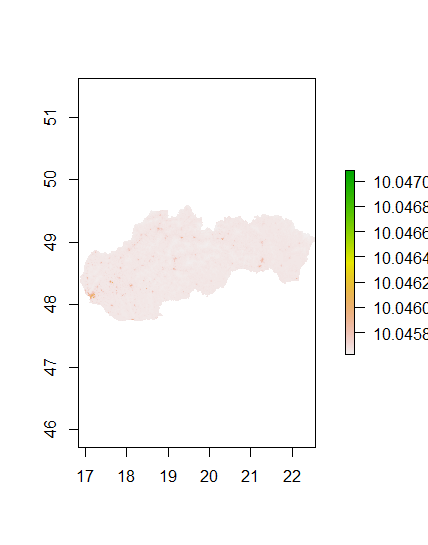
From the results, one can see that for the lower population values the model underpredicted. It expected the population to be greater than it actually was. For the larger populations, at about 85,000 people the model changes to overpredictions. Also, it is interesting to see that the most important variable for the model was the ntl. This makes sense because the brighter an area is at night, the more people who likely live there. With the beginnings of the results coming in, one can transition to the important graphics which predict the population on a map. These are pictured below.

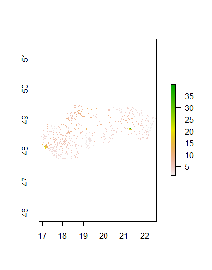
Diff Sums

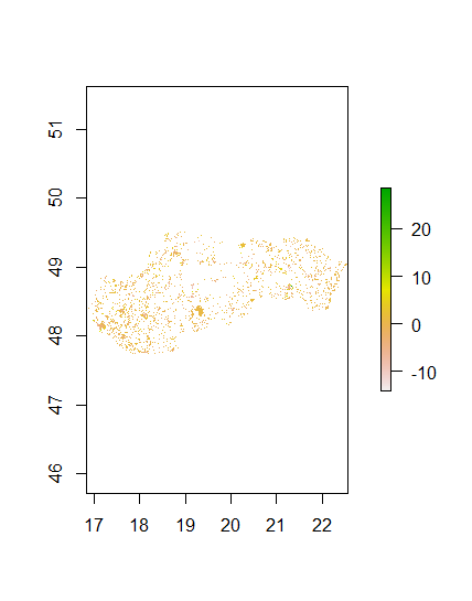
Along with these graphics which display the accuracy of the model are some numbers. When comparing the population sums of the prediction to the actual population, the model is pretty accurate. The predicted value was 5448501 while the acutal value was 5447509. They are less than 1,000 apart. The total difference between the actual and predicted values was 2126206. The average difference per datapoint was 0.0002. The standard deviation was 2.91. To compare this model, the random forest model must now be examined.

The next model to be examined is the random forest. This forest is built of 500 trees and the error for the model can be seen in the image below.

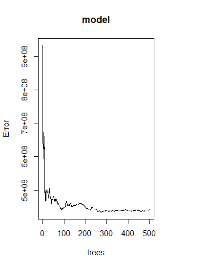
There is a steady decline at the beginning with some slight spikes around 40 trees. The error then decreases around 100 trees where it seems to be near the lowest of the entire model. Around 280 trees the error again decreases and reaches the lowest point in the model. The next image is of the importance of the variables.

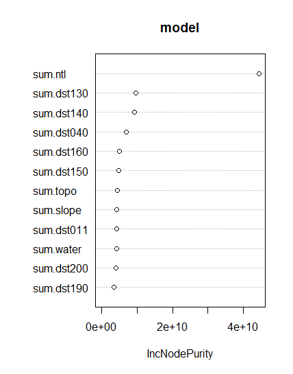
Again, the most important variable is the night time lights. Below are the images of the predictions and the difference between the actual and prediction.

Population Sums

Diff Sums

The total difference between the predicted and acutual populations for the random forests was 2153255, which was significantly larger than the difference for the linear regression. Further The mean was 2.16, meaning on average there was an overprediction of 2 people per data point. The standard deviation was 2.16.

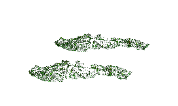
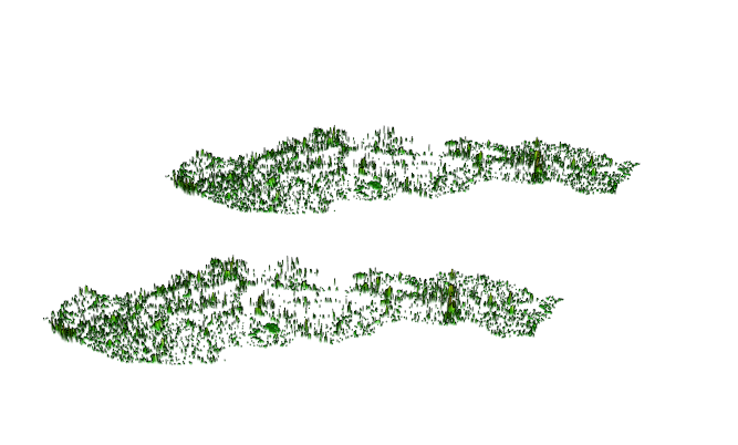
With the two models examined it is important to compare the models. In this comparison it seems the linear regression is the more accurate model. Although the images appear to be very similar, the numbers indicate that there were more errors with the random forest. The same could be said of the raster vision 3D plots, where it is challenging to see the differences. Below is the comparisons for root mean squared error (rmse), mean absolute error (mae), and mean error (me). The bottom image of the country is the linear regression and the top is the random forest.

RMSE

MAE

ME

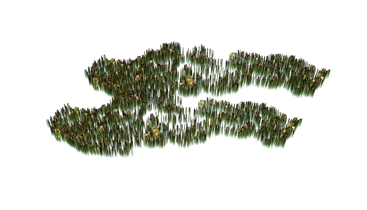
As seen in these images, the mountains areas in the center of the country are overpredicted and the cities, namely Bratislavia and Košice, are overpredicted. This spatial variation makes it more challenging for both models to predict these areas. Overall, the models did a decent job of predicting, but the model that stood out was the linear regression.