DataScience310

For this project, I chose the country of Nepal. This country is in the heart of the Himalayas, just south of China and north of India. This location will be interesting to study for the various regions in relation to the wealth of the individuals in the DHS study.

The first model to be used on this dataset is a penalized logistic regression. For this model, there was a split and sample of the data taken. From here, an evaluation of the AUC - ROC values produced can be done. The “top_model” with the largest AUC was 0.0001 with mean area of .603. Included below is an image of the area under the curve as the penalty increases.

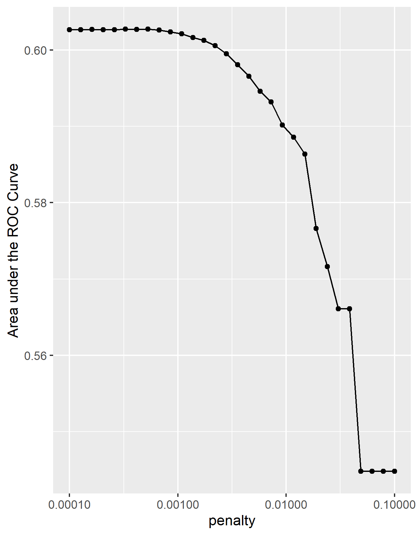
As pictured above, there is a steady line at the beginning hovering at the .603 area under the ROC curve mark. There is even a slight peak from a penalty of .000259 to .000329 but each value’s mean is still .603. This is why I selected the 6th penalty, .000329. From here a ROC plot was completed on the data, which is pictured below.

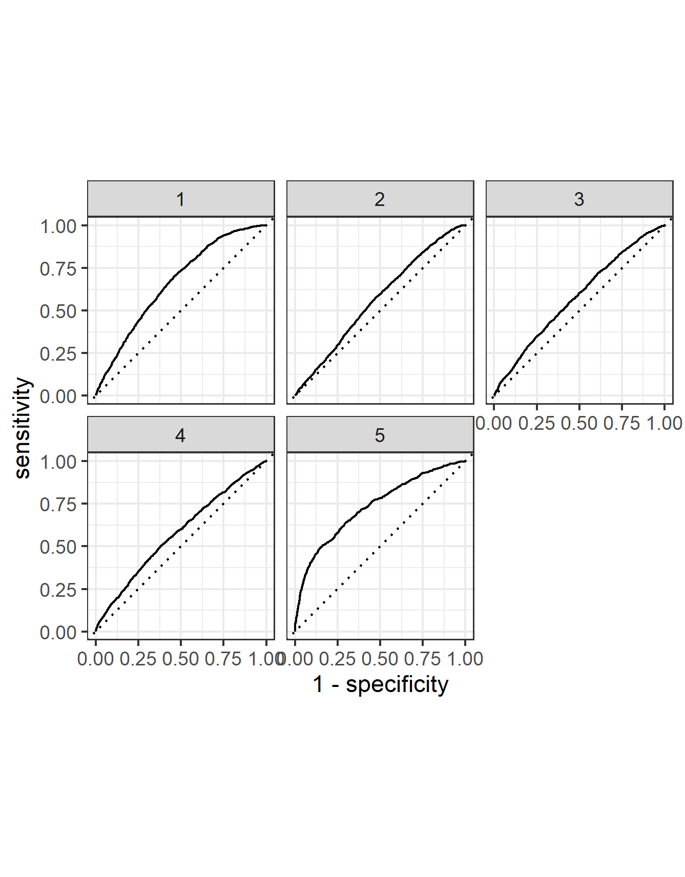
From this image we can see that one wealth outcome stands above the rest in being predicted. The further away from the 45 degree dotted line, or a purely random predictor, the better the predictions. The wealth group 5 is the most accurately predicted. Second is the wealth group 1. The model had a challenging time predicting the middle three wealth groups, which would be expected as they are the most similar to each other and the model likely incorrectly classified between these wealth groups.

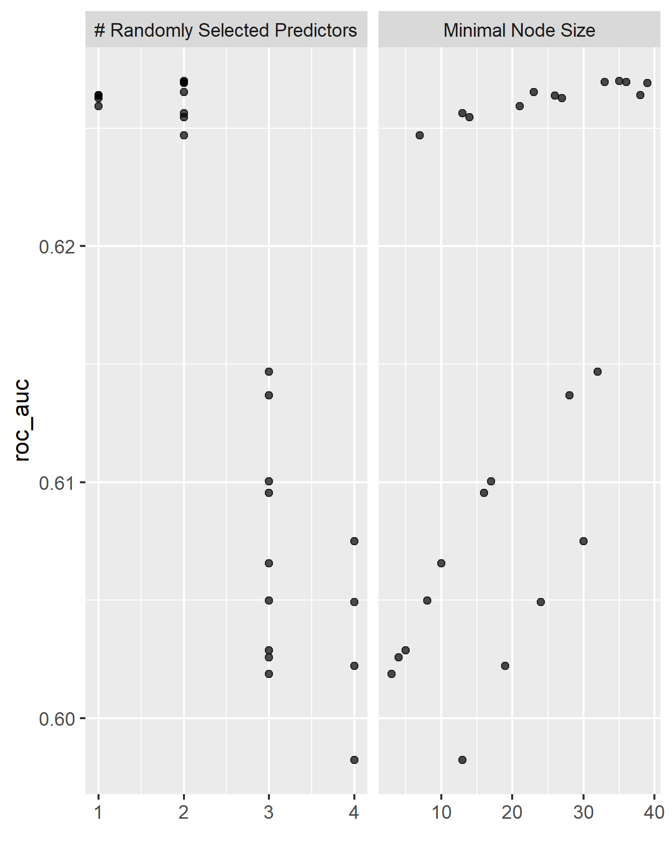
The next model to be interpreted was a random forest. From here the AUC - ROC values for the randomly seleected predictors and the minimal node size were able to be produced. Below is the plot of the results.

The next step was to look at the ROC plots. Below are the curves for each of the wealth groups as well as a comparison to the penalized logistic regression.

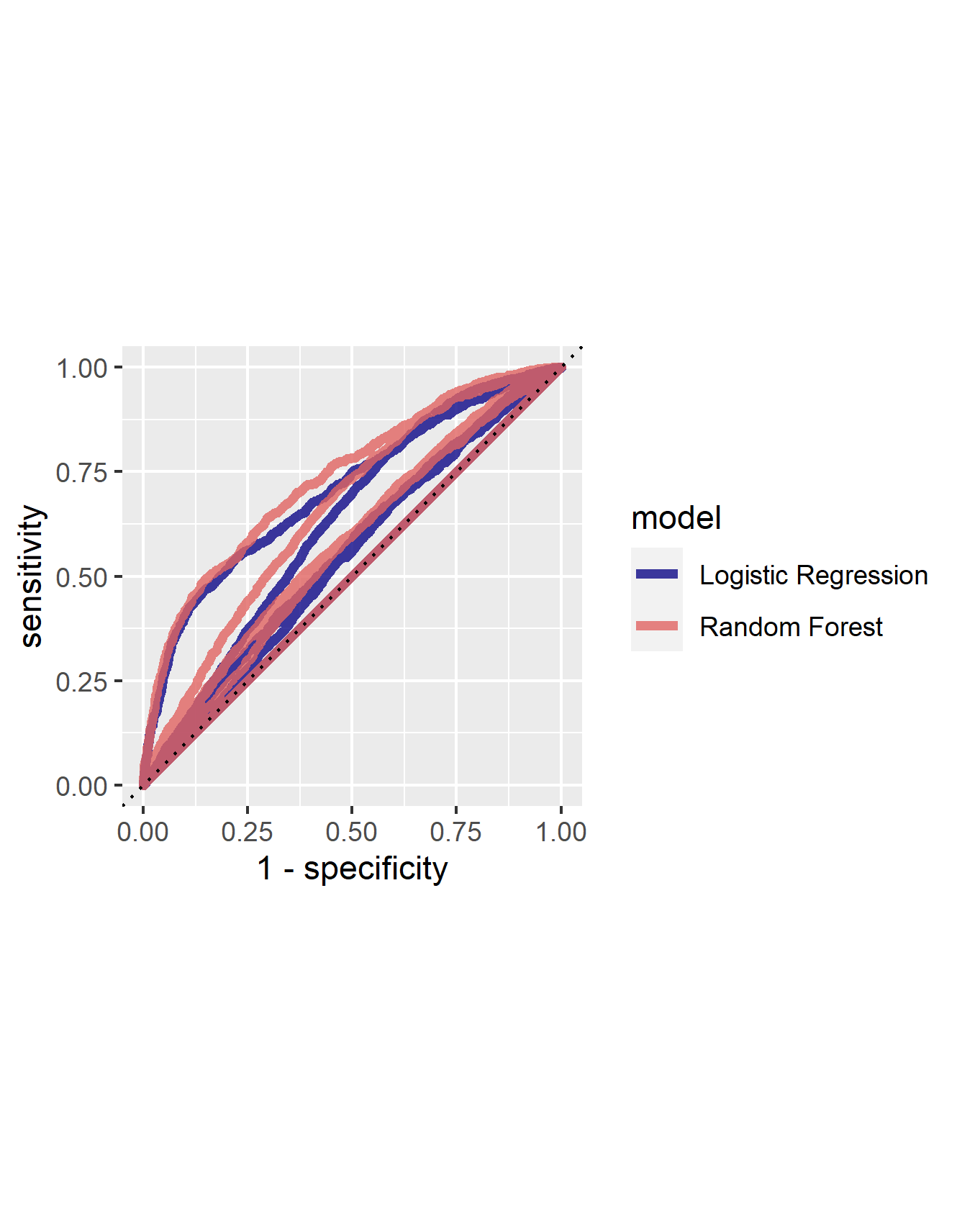
From the first image, we can see that the predictions of the middle three wealth groups, 2, 3, and 4, have improved slightly. Further there has been an increase in both wealth group 1 and 5. This comparison can best be pictured in the second image above where all the red lines, for the random forest, are above their counterpart for the blue lines, the logistic regression. From this interpretation it can be assumed that the random forest does a better job of classifing the wealth groups than the logistic regression. Next, there can be an examination of the relative importance of each feature to the predictive power of the random forest. Below is a graph which displays the importance of each feature.

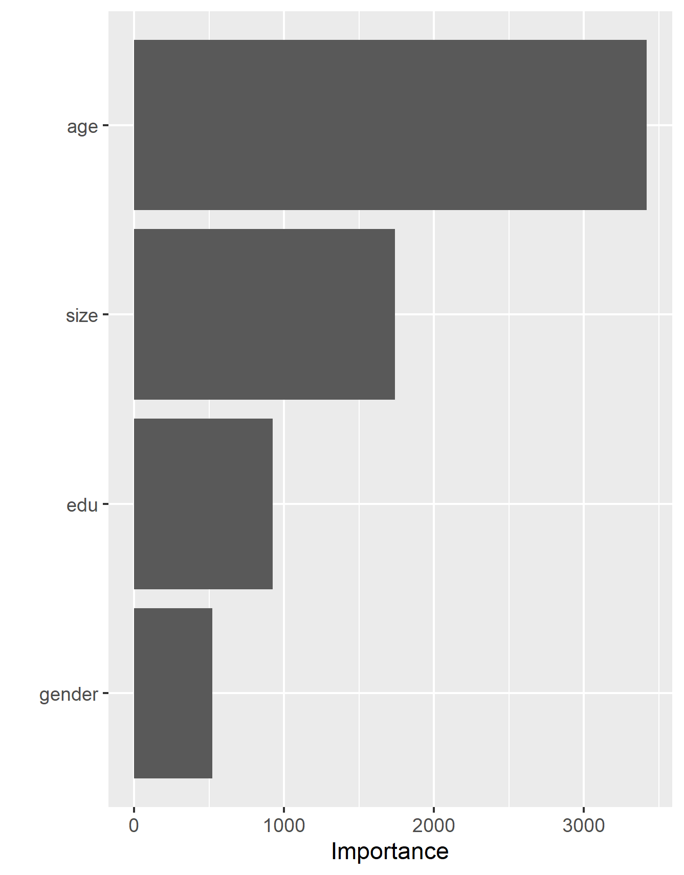
From this image, we can tell that age is the most important predictor of the model, nearly doubling size the second place. The least two important factors are education and gender, with gender being the less important of the two. This suprised me, as I would have expected education to be the most important predictor, but from the data we can see that it is truly age which is the greatest predictor.

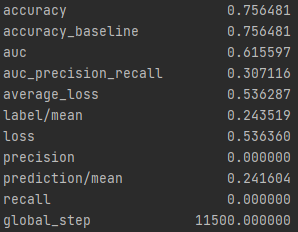
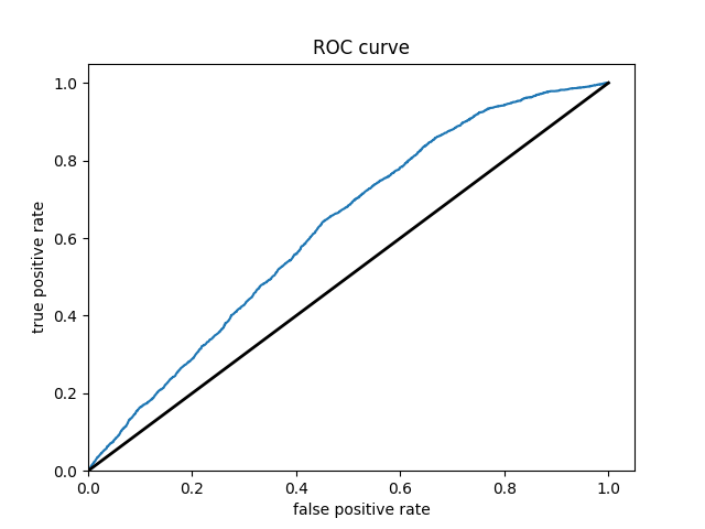
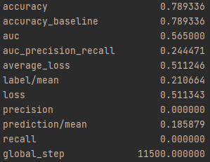
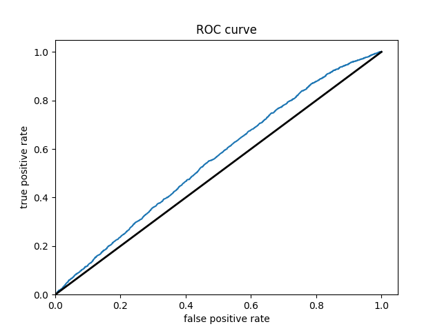
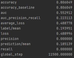
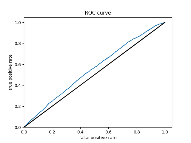
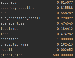
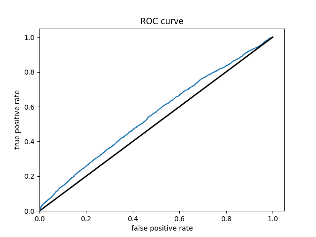
The next model in this report is a logistic regression done in python. One of the first things done on this dataset is setting one wealth in comparison to the other 4. Below are the results of each of the wealth groups and the predictions.

Wealth Group 1

Wealth Group 2

Wealth Group 3

Wealth Group 4

Wealth Group 5

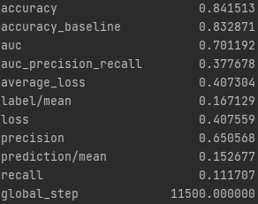
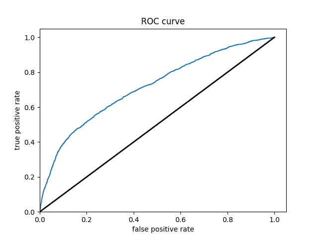
From these results it can be seen that splitting the classifications into one group vs the others greatly improves the accuracy of the model. It is much easier for the classification between in group or out of group rather than chosing from 5 options. The results also improve as one progresses through the groups. Wealth group 5 has nearly a 10% point increase over wealth group 1 in the accuracy.

Further, in this model there was an addition of the derived feature columns selected in order to extend capturing combinations of correlations. I did each of the permuations of the four features, and expended combining the best two features, age and size, it would greatly improve the results. In the end however, the results were not as promising. When done on wealth group 5, the accuracy of the model remained at about the same, but the AUC decreased from above .70 to around .66. The accuracy for each of the groups tells a similar story. None improve through this method. Interestingly for wealth group 3, the AUC decreases below .5 for the combination of gender and education making the model worse than just randomly predicting.

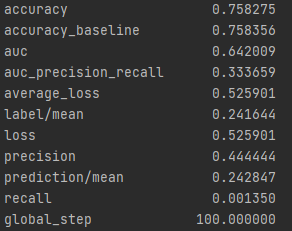
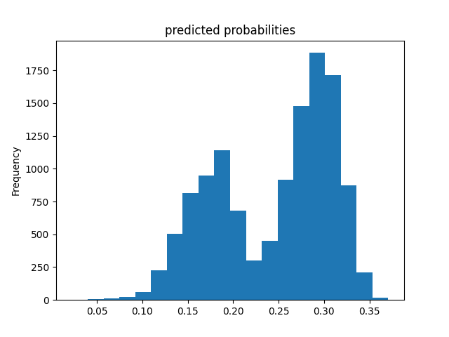
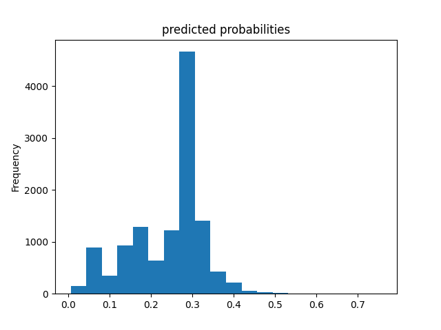
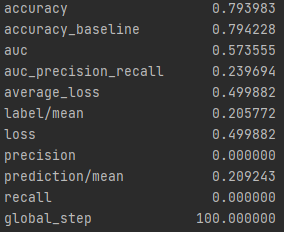
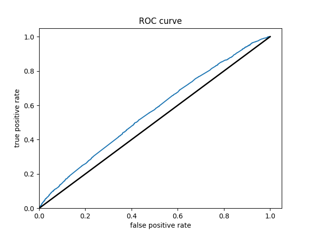
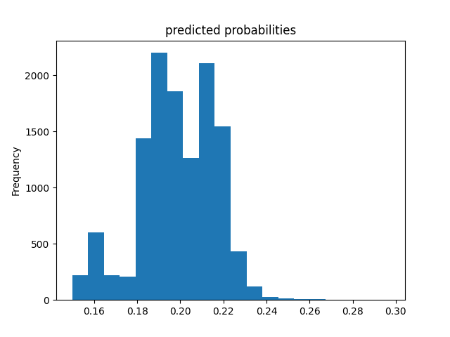
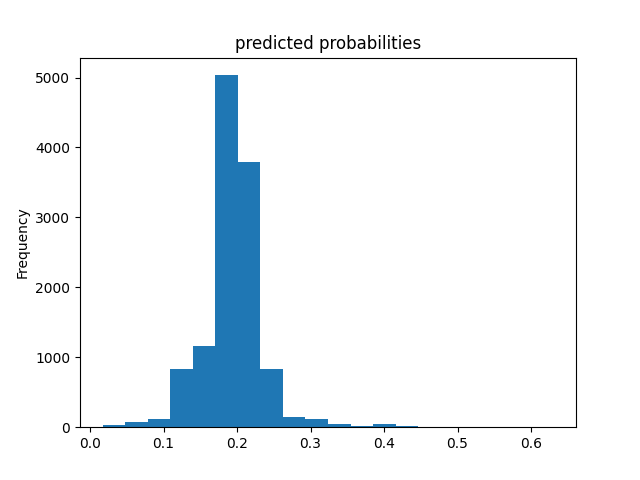
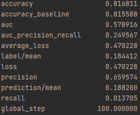
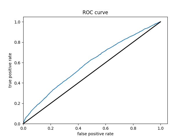
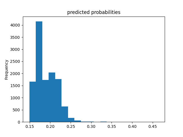
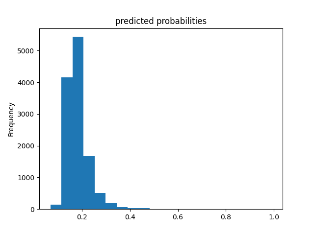
The final model being examined is a gradient boosting model using decision trees. The same 1 versus 4 grouping was done for this model as well. Below are the results for each of the groups.

Wealth Group 1

Wealth Group 2

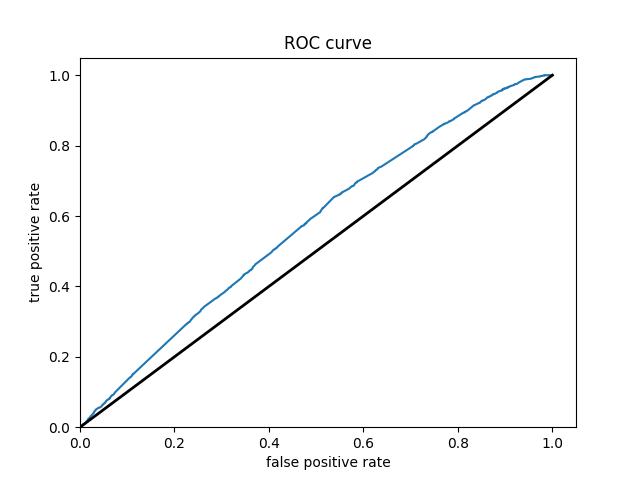
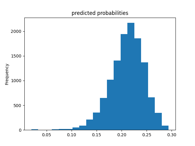
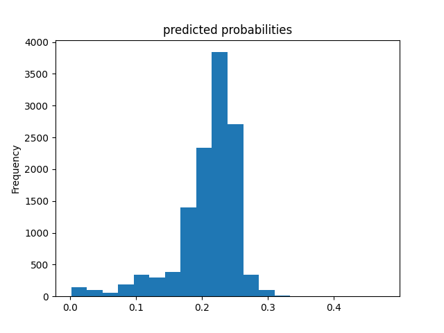
Wealth Group 3

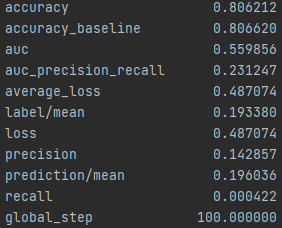
Wealth Group 4

Wealth Group 5

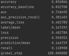
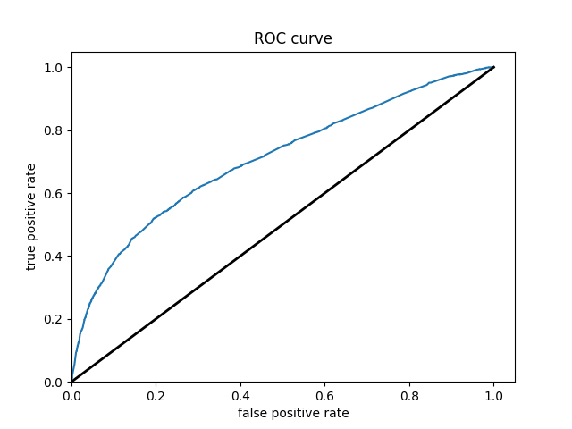
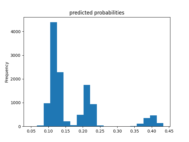
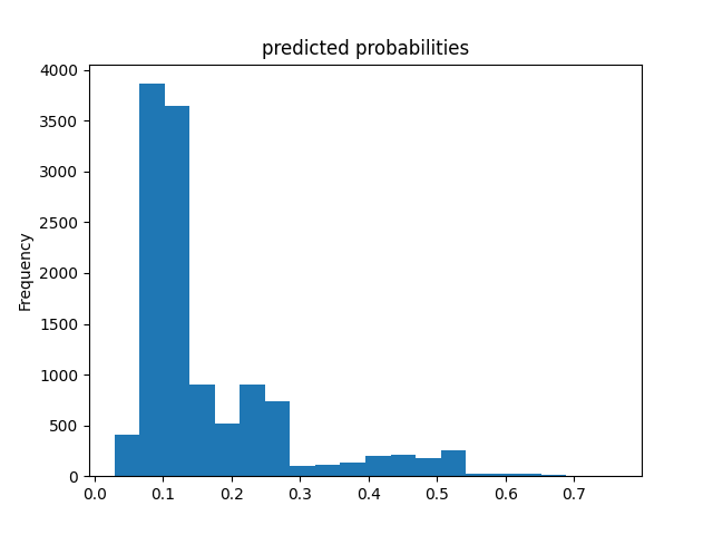
From this information, we can see a steady increase in the accuracy of the model as we get into the higher numbered groups. Like the previous models, the most accurate predictions came for wealth group 5. The results of this model are very similar and comparable to the previous model’s, but slightly more accurate. Further, the AUC values were greater for the gradient boosting model using decision trees.

With all the calculations done, it is time to crown one model as the most impressive. This is a little challenging as each of the graphs are relatively similiar. However, due to the slight improvements over the logistical regression it seems like the gradient boosting model using decision trees is the best of the two. This leaves the random forest and the gradient boosting model using decision trees as the top two. From these it appears that the random forest is superior. The plots of wealth group 3 shows a particularly small AUC for the gradient boosting model. Further, the wealth group 1 has a great AUC for the random forest and is unbeaten. This leaves the random forest as the best model in this report.

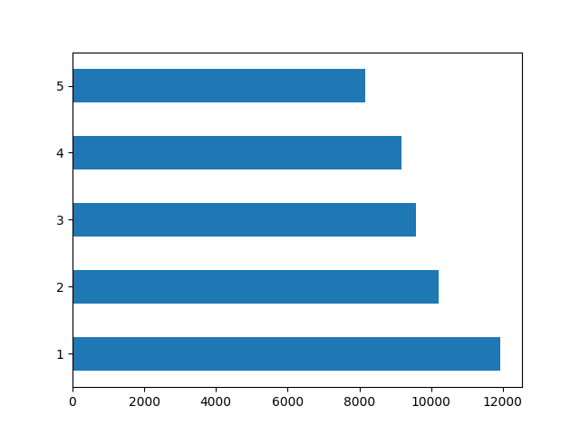
There were no major discrepancies between the five wealth outcomes in the DHS survery dataset. While there were the least number of individuals in wealth group 5, it was not an overwhleming minority. It is likely this smaller grouping which made the accuracy of the models improve as one traverses up the wealth groups. Wealth group 1 is the largest, with group 2 being the second and so on down to 5. This is likely where the improvements in accuracy can be seen. Below is the graphic of the distribution of wealth groups.