DataScience310

Finding a new home can be a challenging endeavor. As a child, I remember riding along with my parents as they would scour neighborhoods looking for their dream house. With the help of new technology the process is becoming less about driving around, and more about what one can find on the internet. Websites, such as Zillow, have become the main way new home buyers have gone through the process of finding their dream home. But how good are the deals on the website, and how can a user know if they are finding the best home for the best value. This has been the goal of this project. To accomplish this task, first data was collected from Zillow, next a model was developed. Afterwards there will be an analysis of the model output and an analysis of the rankings from best to worst deal.

To begin this process, first the data needed to be scraped from Zillow’s website. To do this I completed the task in python. First I chose the city of Boston to be the center of this project. Next, using the urls, each page from Zillow was put into a pandas dataframe. The three columns originally collected from the website were prices, address, and beds. In the beds column were also the values for baths and square feet. Once each of the pages’ data was collected, they were all consolidated into one pandas dataframe. From here the html tags needed to be removed from the columns. I ran into an issue where the price was repeating itself. So if the price of a home was 600,000, it would be stored as 600,000,600,000. With this problem solved, the next issue in the data collection came from the beds column. There were some issues with some of the columns not having all the data required. The rows with missing data were then dropped, leaving me 396 rows, and the data was exported using the .to_csv function. This output was then used in the modelling section of the project.

To prepare the model, some things still needed to be completed on the data. After importing the csv file into a new modeling python file, the prices and square footage were normalized. Each of the prices were divided by 100,000 and each of the square feet were divided by 1,000. This hoped to reduce the bias in these columns during the model fitting. The model itself is a tensorflow keras sequential model with an input shape of 3 and an activation = ‘softplus’. The softplus was used because there were some errors in testing where a negative output would result, the softplus mandates that the predicted value be greater than 0. The three input layers are beds, baths, and square feet. The y variable, or the predicted variable, was the prices of the homes. The model was compiled with an optimizer of stochastic gradient descent and a loss function of mean squared error. From here the model was fit over 1,000 epochs. From this, I was able to gain the model output and begin predicting the prices of homes.

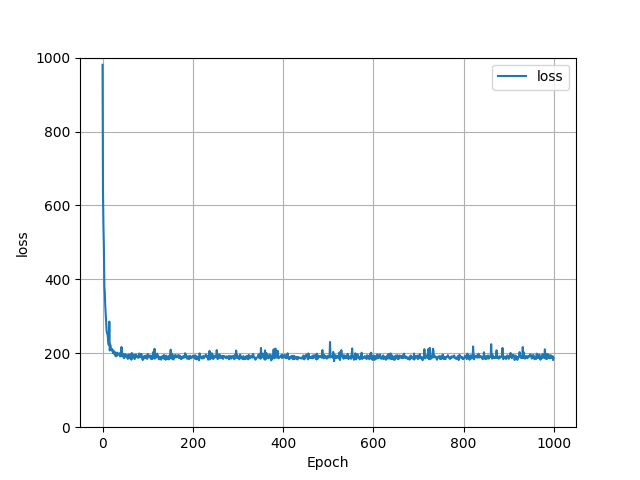
The model was now ready to output data. For the last run through the data, the loss was 217.4033. The entire history of the loss function can be seen in the graph above. As one can see, there was a steady decline at the start, but after around 10 epochs it hovers around the 200 mark and goes up and down from there frequently. The mean squared error of the entire dataset was 1881421385469.6182.

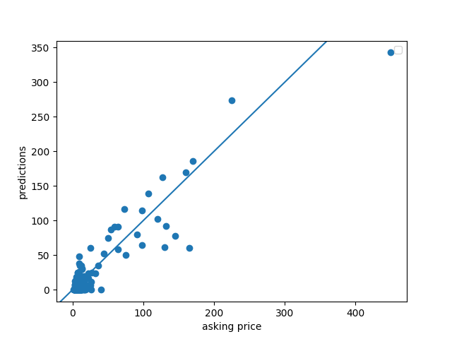
The next graphic is the predicted vs asking price graph. For this image, the line demonstrates a 1:1 ratio if the value was perfectly predicted. Any point to the left was over predicted, and any point to the right was underpredicted. The main outlier is a home which is valued at $45,000,000 which the predicted value was nearly $35,000,000. The majority of the data was underpredicted.

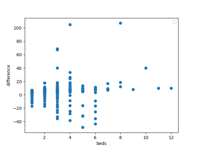
Finally we come to the best and worst predictions from this dataset. I found that the data with 1 or 2 beds were relatively effective at being predicted. This can be seen with the graphic above. This graph demonstrates the number of beds in relation to the difference in price. However, when the number of beds increased, the predicted failed to be as accurate both for good deals and bad deals. This can be seen in the larger spread of data points from 3 or greater beds. The model was successful at predicting homes with 7 beds, with a consistant lean on underpredicting. Of the 10 best deals, each had at least 3 bedrooms with the average being 5.1 bedrooms. The MSE of these points was 37677214112014.48. While a large error still existed for the worst 10 deals, the MSE was better at 12952392933633.336. These points also had at least 3 bedrooms in their homes. In comparison, the 10 best priced data only had a MSE of 3170155074.7586985 and included 6 homes with either 1 or 2 bedrooms.

This project looked at the effectiveness of a model to predict the prices of homes. There were some issues with collecting the data, but overall the model did a good job of predicting homes with 1 or 2 bedrooms. After collecting and preparing the data, a model was created. From there the results of the machine were able to be examined by looking at the outputs and the best and worst prediction. Perhaps if my parents had a tool like this, they would have gotten a better deal.