DataScience310

For the next section of the module, two models were looked at; a linear regression and a random forest. Again the country selected was Slovakia as it was much smaller than Nepal and thus the data was much easier to work with for the module. The set up for these models was much the same as for the previous part. The data was imported and saved as rasters or dataframes. The columns were given names and then the data was exact_extracted. To start off the comparison linear regression will be looked at first.

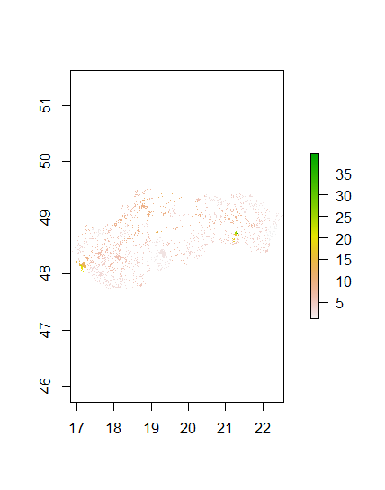
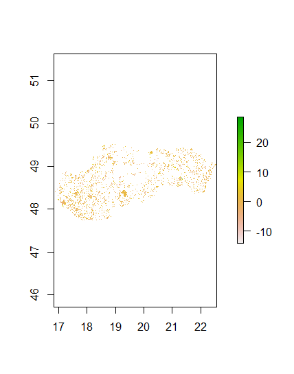
In the linear regression model the same steps as the last section of the module was done to prep the data and get the model to predict values. The results for the cellStats(population_sums, sum) was 5448501 while the results for the sum(svk_adm2$pop20) was 5447509. These results were pretty close with less than a 1000 person difference. Below are the plots for the population_sums and diff_sums.

Population Sums

Diff Sums

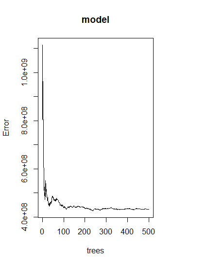
With the linear regression model complete, the next model being examined is a random forest. The same data was used, and the model was run. Below is the image of the error against the number of trees.

As one can see, there is a steady drop as the number of trees increase until around 50 trees. Then there is a slight spike before going back down again and essentially leveling out. The lowest point seems to be around 240 trees. Next, the most important varaibles will be examined.

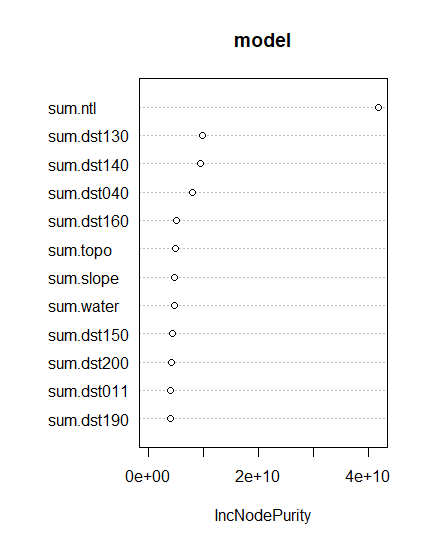
From this model it is clear again that ntl is the most important variable with each of the others being significantly less important. Next, the population sums and actual population are being compared. The cellStats(population_sums, sum) for the random forest was 5448499, which was two people closer than the linear regression. Finally the maps of the population sums and difference sums will be displayed.

Population Sums

Diff Sums